In my last post, I’ve talked about Head-Related Transfer Functions and how to use them to create virtual, binaural audio. In this post I’ll show how to write a stereo panner that uses HRTF to position a mono source in 3D space. I’ll implement it in JavaScript with the use of Web Audio API. Although Web Audio API already offers a stereo panner that uses HRTF, it is not of the best quality and provides no way of choosing the Head-Related Transfer Function to use which results in an effect that may not sound realistic for everyone. The ability to choose that particular HRTF which results in a best experience is very important. Another reason that i decided to use Web Audio API for implementation is accessibility – all you need is a web browser. The algorithm I’m about to present can be easily ported to any other language.
Some theory first
The process of using HRTF to create binaural sound from a mono source is simple: We convolute the mono signal with Head-Related Impulse Response (HRIR) for the left and right ear respectively. Since HRIR is different for each direction we need to select appropriate HRIR depending on the position we want our source to be.
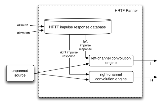
Diagram illustrating the basic process of panning using HRTF
There are many databases available. Google “HRTF database” and you’ll get many websites from which you can download sets of HRTF impulse responses. The most popular and very well documented one is CIPIC HRTF Database. It provides HRIR for over 40 subjects with respective data about physical properties (detailed head and ear dimensions) and also comes with a Matlab script to load, visualize and listen to all HRTFs.
Regardless of the database chosen, it is necessary to understand the coordinate system our database is using. HRTF (HRIR) is a function of an angle (direction) besides time, obviously. The angle is most of the time specified a a pair of azimuth and elevation. What angles azimuth and elevation are exactly depends on the coordinate system. CPIC database uses so-called Interaural-Polar Coordinate System:

Interaural-Polar Coordinate System used by the CIPIC database compared to the common Spherical coordinate system.
In this coordinate system, elevation is the angle from the horizontal plane to a plane through the source and the x axis (called the interaural axis) and the azimuth is then measured as the angle over from the median plane. So, for example, the point (azimuth = 0, elevation = 0) is the point directly ahead, (azimuth = 90, elevation = 0) is directly to the right, (azimuth = 0, elevation = 180) is behind and so on…HRTFs from the CIPIC database are recorded at elevations from -45 deg to 230.625 deg at constant 5.625 degree intervals and azimuths from -80 to 80 (image below)
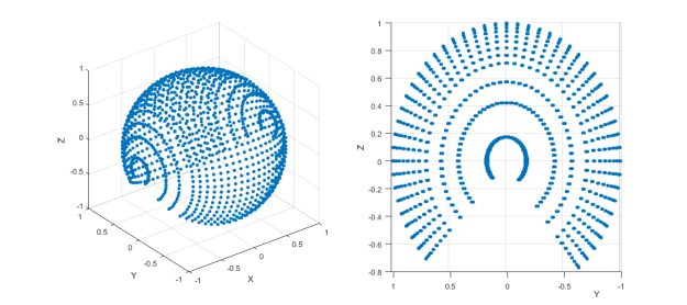
Visualization of points at which HRIR from CIPIC are recorded.
There is a fundamental problem that needs to be solved: HRIRs are, naturally, recorded for a finite set of points. On top of that, those points almost never cover the full sphere around the head. It doesn’t make sense to make a panner that allows to position the source only at points for which HRIR we have are recorder. In order to be able to pan a moving source, without audible “jumps” we need some method of interpolation.
One approach could involve taking impulse responses from neighbor points and sum them with weights proportional to distance from the interpolated point. If we restricted those weights to sum to 1, we would have implemented a kind of Vector Base Amplitude Panning (VBAP). This is proven to give good results, especially in the case of surround sound systems, but for HRTF interpolation, a better method exists.
The method is described here: http://scitation.aip.org/content/asa/journal/jasa/134/6/10.1121/1.4828983 Firstly, the 3D triangulation is performed on the original set of points, which are triplets of (azimuth, elevation, distance). As a result the points become vertices of tetrahedrons. To obtain an interpolated HRIR at point X, we need to find a tetrahedron enclosing that point and sum HRIRs from it’s vertices with weights corresponding to barycentric coordinates of X. Therefore the interpolated HRIR is a barycenter of the four neighbor HRIRs. In case our HRIR data is measured at constant distance ( is only a function of azimuth and elevation) there is one dimension less and we search through triangles instead of tetrahedrons, in a 2D triangulation and sum only three HRIR components. HRTFs from CIPIC are function of only azimuth and elevation so we will be dealing with the 2D case, but the algorithm can very easily be scaled to add another dimension basing on the aforementioned paper.
Implementation
Let’s start by defining a class that will load and store the impulse response and triangulation and also perform the interpolation. I’ll call it “HRTF Container”. Instance of this class is what each panner will refer to.
function HRTFContainer() {

	var hrir =  {};
	var triangulation = {};

	this.loadHrir = function(file, onLoad) {
	        // ...
	}

	this.interpolateHRIR = function(azimuth, elevation) {
	        // ...
	}
}
We’re now going to define it’s two methods, starting with
Loading impulse response
The HRIR from CIPIC database is stored in .mat file format. There are few variables but only one is an actual impulse response, stored as
2[left and right] x 25[azimuths] x 50[elevations] matrix. Those 25 azimuths and 50 elevations form a grid pictured above and as You can see they don’t form a complete sphere around the head. If we are to use the method of interpolation that base on a triangulation, it would be better to not have holes. Also, the panner should be able to pan the source in any desired direction. Therefore we need to extrapolate the missing data. The most important points are directly to the left and right, those are +/- 90 azimuth. Also, points below the head are missing. This obviously comes from the fact that the source would need to be in a person’s body. This is the reason we very rarely, almost never, listen to the sound coming directly from below. It is a question whether it makes sense to create a panner that offers such an option. If it does, the result won’t be realistic anyway. However, i decided to do that and extrapolate the “directly below” direction. Why? Because of practical reasons. It will be easier to have a panner that covers the full sphere since we won’t have to restrict the direction – our panner will work for every possible angle. The effect won’t be as realistic as but it’s still better than none.
Here is the script that exports the hrir data from the .mat file to the binary (.bin) format that I’ll load into JavaScript. The points directly to the left (+/- 90 azimuths) are simply an arithmetic mean of the points for +/- 80 azimuth. Points below (elevation = 270 = -90) are a weighted mean of points for elevation = -45 and 230.625.
The code to load the data from the .bin file is pretty straightforward, as long as the layout of the binary data is known:
this.loadHrir = function(file, onLoad) {
	var oReq = new XMLHttpRequest();
	oReq.open("GET", file, true);
	oReq.responseType = "arraybuffer";
	oReq.onload = function(oEvent) {
		var arrayBuffer = oReq.response;
		if (arrayBuffer) {
			var rawData = new Float32Array(arrayBuffer);
			var ir = {};
			ir.L = {};
			ir.R = {};
			var azimuths = [-90, -80, -65, -55, -45, -40, -35, -30, -25, -20, -15, -10, -5, 0,
                5, 10, 15, 20, 25, 30, 35, 40, 45, 55, 65, 80, 90];
			var points = [];

			var hrirLength = 200;
			var k = 0;
			for (var i = 0; i < azimuths.length; ++i) {
				azi = azimuths[i];
				ir['L'][azi] = {};
				ir['R'][azi] = {};

				// -90 deg elevation
				ir['L'][azi][-90] = rawData.subarray(k, k + hrirLength);
				k += hrirLength;
				ir['R'][azi][-90] = rawData.subarray(k, k + hrirLength);
				k += hrirLength;

				points.push([azi, -90]);
				// 50 elevations: -45 + 5.625 * (0:49)
				for (var j = 0; j < 50; ++j) {
					var elv = -45 + 5.625 * j;
					ir['L'][azi][elv] = rawData.subarray(k, k + hrirLength);
					k += hrirLength;
					ir['R'][azi][elv] = rawData.subarray(k, k + hrirLength);
					k += hrirLength;
					points.push([azi, elv]);
				}

				// 270 deg elevation
				ir['L'][azi][270] = rawData.subarray(k, k + hrirLength);
				k += hrirLength;
				ir['R'][azi][270] = rawData.subarray(k, k + hrirLength);
				k += hrirLength;
				points.push([azi, 270]);
			}
			hrir = ir;
			triangulation.triangles = Delaunay.triangulate(points);
			triangulation.points = points;
			if (typeof onLoad !== "undefined")
				onLoad();
		}
		else {
			throw new Error("Failed to load HRIR");
		}
	};
	oReq.send(null);
}
Hrir is stored as float array, each HRIR is 200 samples long. With each loaded hrir we store the (azimuth, elevation) point and at line 48 the triangulation from those points is performed. I’ve used the Delaunay triangulation by ironwallaby.
Interpolation
This is a direct implementation of the algorithm described in the paper mentioned earlier.
We iterate through all the triangles in the triangulation. The triangle enclosing the point we want to interpolate is found when all the barycentric weights (g1, g2 and g3) are non-negative. The interpolated HRIR is a weighted sum of the 3 HRIRs corresponding to vertices of that triangle:
this.interpolateHRIR = function(azimuth, elevation) {
	var triangles = triangulation.triangles;
	var points = triangulation.points;
	var i = triangles.length - 1;
	var A, B, C, X, T, invT, det, g1, g2, g3;
	while (true) {
		A = points[triangles[i]]; i--;
		B = points[triangles[i]]; i--;
		C = points[triangles[i]]; i--;
		T = [A[0] - C[0], A[1] - C[1],
			 B[0] - C[0], B[1] - C[1]];
		invT = [T[3], -T[1], -T[2], T[0]];
		det = 1 / (T[0] * T[3] - T[1] * T[2]);
		for (var j = 0; j < invT.length; ++j)
			invT[j] *= det;
		X = [azimuth - C[0], elevation - C[1]];
		g1 = invT[0] * X[0] + invT[2] * X[1];
		g2 = invT[1] * X[0] + invT[3] * X[1];
		g3 = 1 - g1 - g2;
		if (g1 >= 0 && g2 >= 0 && g3 >= 0) {
			var hrirL = new Float32Array(200);
			var hrirR = new Float32Array(200);
			for (var i = 0; i < 200; ++i) {
				hrirL[i] = g1 * hrir['L'][A[0]][A[1]][i] +
					g2 * hrir['L'][B[0]][B[1]][i] +
					g3 * hrir['L'][C[0]][C[1]][i];
				hrirR[i] = g1 * hrir['R'][A[0]][A[1]][i] +
					g2 * hrir['R'][B[0]][B[1]][i] +
					g3 * hrir['R'][C[0]][C[1]][i];
			}
			return [hrirL, hrirR];
		}
		else if (i < 0) {
			break;
		}
	}
	return [new Float32Array(200), new Float32Array(200)];
}
Panner
Now that we have a way to load HR impulse response and interpolate it for every direction desired, we can finally code the actual panner. For the rest of this post I’ll assume You have basic knowledge of the Web Audio API, which means You read at least the Introduction section of the official documentation. :)
The heart of the HRTF Panner is the convolution process. Web Audio API offers a ConvolverNode interface for that. Since we need to convolve with HRIR for both ears (left and right channel), we need two convolvers (with one-channel buffer each) or one convolver using a two-channel buffer. For convenience, I’ll go with the latter:
function HRTFConvolver() {
	this.convolver = audioContext.createConvolver();
	this.convolver.normalize = false;
	this.buffer = audioContext.createBuffer(2, 200, audioContext.sampleRate);
	this.convolver.buffer = this.buffer;
	this.gainNode = audioContext.createGain();

	this.convolver.connect(this.gainNode);

	this.fillBuffer = function(hrirLR) {
		var bufferL = this.buffer.getChannelData(0);
		var bufferR = this.buffer.getChannelData(1);
		for (var i = 0; i < this.buffer.length; ++i) {
			bufferL[i] = hrirLR[0][i];
			bufferR[i] = hrirLR[1][i];
		}
		this.convolver.buffer = this.buffer;
	}
}
Nothing extraordinary…we create the two-channel buffer with length of 200 samples (that’s the length of HRIR from CIPIC) and then set the convolver to use that buffer. Before it is done however, we must set the ConvolverNode.normalize attribute to false, so that the Web Audio API algorithms does not normalize our impulse response. It is necessary because HRIRs from the CIPIC database are already normalized. I also create a GainNode and connect the convolver to it. I’ll explain the purpose of that GainNode in a bit. In the fillBuffer method we fill buffer with new impulse response via “pointers” to the underlying arrays (the getChannelData() method). At line 17 we need to set the buffer again because of the fact that call to getChannelData apparently resets the ConvolverNode.buffer attribute.
Now, if we were simply to change the convolver’s impulse response we would get audible glitches/cracks, caused by a rapid change of the filter. To avoid that we would need to add the last 200 (length of the impulse response) filtered samples from the output (so called tail) to the input and that’s simply not possible without creating a processor script, which would deal with raw samples causing a massive drop in performance, defeating the purpose of using Web Audio API in the first place. So the solution is like this: create two convolvers , update only one of them (let’s call it the target convolver) and crossfade between the two. After crossfading completes, swap the references:
function HRTFPanner(audioContext, sourceNode, hrtfContainer) {

	function HRTFConvolver() {
		// ...
	}

	var currentConvolver = new HRTFConvolver();
	var targetConvolver = new HRTFConvolver();

	this.update = function(azimuth, elevation) {
		targetConvolver.fillBuffer(hrtfContainer.interpolateHRIR(azimuth, elevation));
		// start crossfading
		var crossfadeDuration = 25;
		targetConvolver.gainNode.gain.setValueAtTime(0, audioContext.currentTime);
		targetConvolver.gainNode.gain.linearRampToValueAtTime(1, audioContext.currentTime + crossfadeDuration / 1000);
		currentConvolver.gainNode.gain.setValueAtTime(1, audioContext.currentTime);
		currentConvolver.gainNode.gain.linearRampToValueAtTime(0, audioContext.currentTime + crossfadeDuration / 1000);
		// swap convolvers
		var t = targetConvolver;
		targetConvolver = currentConvolver;
		currentConvolver = t;
	}
}
At line 11 we fill the target convolver’s buffer with the interpolated impulse response. At line 15 we schedule the gain of the target convolver’s to raise from 0 to 1 and the opposite for the current convolver at line 17. Then, we swap the references. This is very similar to the Double-Buffer pattern used by GPUs, except for the crossfading part. In the code above the crossfading time is 25 milliseconds. That is enough to avoid audible glitches, at least in theory. I’ve tested it on many signals and this value seems to be enough but it may not always be the case. The longer the time, the more save we are, however at the cost of the delay caused by the transition.
The last thing, which is not necessary but highly desirable, is a crossover. The purpose of the crossover in a HRTF Panner is to don’t spatialize lowest frequencies. Those are in their nature non-directional: hearing a deep bass coming only from one direction is very unnatural to hear. Therefore we can separate the lowest frequencies of the source signal and send them directly to the output and convolute only the frequencies above the cutoff frequency. To do that we can use the BiquadFilterNode interface:
function HRTFPanner(audioContext, sourceNode, hrtfContainer) {

	function HRTFConvolver() {
		// ...
	}

	var currentConvolver = new HRTFConvolver();
	var targetConvolver = new HRTFConvolver();

	var loPass = audioContext.createBiquadFilter();
	var hiPass = audioContext.createBiquadFilter();
	loPass.type = "lowpass";
	loPass.frequency.value = 200;
	hiPass.type = "highpass";
	hiPass.frequency.value = 200;

	var source = sourceNode;
	source.channelCount = 1;
	source.connect(loPass);
	source.connect(hiPass);
	hiPass.connect(currentConvolver.convolver);
	hiPass.connect(targetConvolver.convolver);
This is almost all that there is to it. Last thing we need is to define the methods for connecting the panner to the output (so it can be used kind of like the native AudioNode interface) and some other methods, like changing the source or crossover frequency:
	/*
		Connects this panner to the destination node.
	*/
	this.connect = function(destination) {
		loPass.connect(destination);
		currentConvolver.gainNode.connect(destination);
		targetConvolver.gainNode.connect(destination);
	}

	/*
		Connects a new source to this panner and disconnects the previous one.
	*/
	this.setSource = function(newSource) {
		source.disconnect(loPass);
		source.disconnect(hiPass);
		newSource.connect(loPass);
		newSource.connect(hiPass);
		source = newSource;
	}

	/*
		Sets a cut-off frequency below which input signal won't be spatialized.
	*/
	this.setCrossoverFrequency = function(freq) {
		loPass.frequency.value = freq;
		hiPass.frequency.value = freq;
	}
The full code, along with the example can be found at my repo: https://github.com/tmwoz/hrtf-panner-js
I’ve also written a browser application that showcases the whole CIPIC database here: https://github.com/tmwoz/binaural-hrtf-showcase


